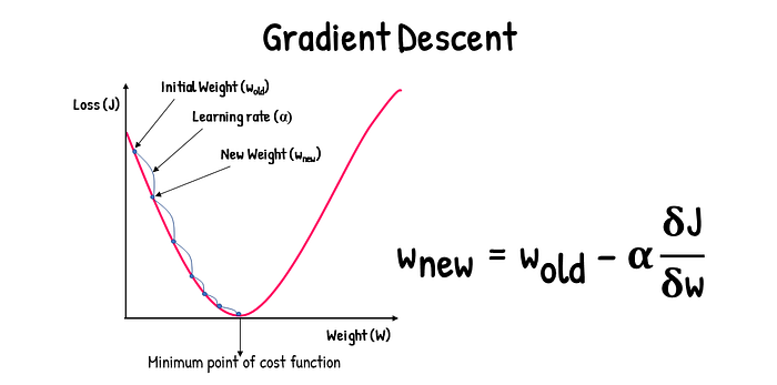
In the realm of machine learning, the precision with which we can fine-tune the coefficients of our model’s variables is paramount. This blog post delves into one of the fundamental optimization methods used in machine learning: Gradient Descent. Our focus will be to unravel the logic behind this technique and explain why it’s so critical for building effective models.

What is Gradient Descent?

Gradient Descent is an optimization algorithm used to minimize the cost function in a machine learning model. The essence of the cost function lies in the difference between the predicted values and the actual values. The smaller this difference, the more accurate our model is.

How Does Gradient Descent Work?

Imagine starting at a random point on a graph of the cost function. Gradient Descent involves drawing a tangent at this point and determining its slope through differentiation. The slope or gradient tells us the rate at which one variable changes with respect to another, analogous to how the derivative of position with respect to time gives velocity, and the derivative of velocity gives acceleration.

Here’s the step-by-step process:

• Start at a random point: Select a random point on the cost function graph as the starting point.
• Calculate the gradient: At this point, compute the gradient of the cost function. The gradient is essentially the derivative and indicates the direction of the steepest ascent.
• Update the coefficients: Adjust the coefficients of your model in the direction that results in the steepest descent in the cost function. This adjustment is made using the formula:

θnew​=θold​−α×∇J(θ)

where θ represents the coefficients, α is the learning rate, and ∇J(θ) is the gradient of the cost function at θ.

• Repeat until convergence: This process is repeated iteratively until the cost function reaches a minimum or is sufficiently close to a minimum.

Importance of the Learning Rate

The parameter α in the formula is known as the learning rate. It determines the size of the steps we take on each iteration of Gradient Descent:

• A high learning rate can lead the algorithm to overshoot the minimum, possibly diverging.
• A low learning rate will result in smaller steps, which can slow down the convergence and increase the computational cost.

Choosing the right learning rate is crucial, as it influences the efficiency and effectiveness of the model training.

Key Takeaways

Gradient Descent is a powerful optimization method in machine learning that helps determine the optimal coefficients of the independent variables by minimizing the difference between predicted and actual values using derivatives. It’s an iterative technique that improves the model with each step, moving towards the most accurate predictions possible.

Note: In the cost function notation, the ‘m’ value denotes the number of observations in the dataset, which should not be confused with ‘m’ used in the gradient formula.

In conclusion, understanding and implementing Gradient Descent allows for precise model tuning and can significantly impact the performance of predictive models in machine learning.

Whether you are a seasoned data scientist or a newcomer to machine learning, mastering Gradient Descent will equip you with a fundamental tool for model optimization. Keep experimenting with different learning rates and starting points to see how they affect the performance of your models. Happy modeling!